Predicting Customer Lifetime Value (CLV) using Probabilistic Model

9 min readApr 14, 2024

This is the next part of my article about "Unlocking Customer Segmentation Insights by combining RFM analysis with K-Means Clustering."

If you haven't read it, you can read it here:

https://medium.com/@ishla/unlocking-customer-segmentation-insights-combining-rfm-analysis-with-k-means-clustering-45bdc6bf8555

What is Customer Lifetime Value (CLV)?

Customer lifetime value (CLV) is a customer's total revenue or profit over their relationship with the business. Simply speaking, it's a metric to measure the total amount of money a customer has spent (or is expected to spend) on your products and services throughout their lifetime as a customer. — Gartner

What benefits the Customer Lifetime Value Model?

It guides who to target, what to sell, and how to communicate.
Increase profits over time.
Improved customer retention and reduced churn.
Reduce customer acquisition costs.
Better decision-making and forecasting.

Types of Customer Lifetime Value

There are two models that companies will use to measure customer lifetime value.

Historical CLV: The model looks at past data and makes a judgment on the value of customers based on previous transactions alone, without any attempt to predict what those customers will do next.
Predictive CLV: The model forecasts the buying behavior of existing and new customers using regression or machine learning.

At this moment, I'll guide you in implementing the predictive CLV model using the BG-NBD Model and Gamma-Gamma Model.

What is the BG-NBD Model?

Geometric Beta Distribution / Negative Binomial known as the BG-NBD Model. Also known as "Buy Till You Die," it predicts the expected number of transactions in a certain period. This model can answer the following questions:

How many transactions will occur in the next week?
How many transactions will occur in the next three months?
Which customers will make the most purchases in the next two weeks?

What is the Gamma-Gamma Model?

The Gamma-Gamma model predicts the average profit earned from each customer. After modeling the overall average profit, the expected average profit for each customer is obtained.

A customer's monetary value (the total number of customer transactions) will be randomly distributed around their average transaction value.
Average transaction value may change over time between customers but does not change for customers.
The average transaction value will be distributed gamma to all customers as gamma.

High-level overview CLV Model

Create CLV Model

I will provide detailed guidance on implementing the CLV Model using Python. This will include step-by-step instructions to help you understand and execute each process.

Import Libraries

#Import Libraries
import pandas as pd  # For data manipulation and analysis
import numpy as np   # For numerical operations on arrays
import matplotlib.pyplot as plt  # For creating plots and graphs
import seaborn as sns  # For making attractive and informative statistical graphics
from datetime import timedelta  # For handling time-based calculations
import plotly.express as px  # For interactive visualizations
import datetime as dt # for manipulating dates and times
import lifetimes # Python library for analyzing customer lifetime value

Load Dataset

I use an Online Retail data set that contains all the transactions occurring for a UK-based and registered, non-store online retailer between 01/12/2009 and 09/12/2011. The company mainly sells unique all-occasion giftware, and many of its customers are wholesalers.

You can access the dataset using this link: https://archive.ics.uci.edu/dataset/502/online+retail+ii.

# Load a CSV file into a DataFrame
df = pd.read_csv('Online_Retail.csv', encoding='ISO-8859-1')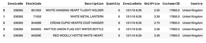

Fitting and testing the BG/NBD model

First, we must split our dataset into calibration and observation (holdout). The first period will be used to fit the model, and the second period will be used to test the model.

In the dataset, we have 373 days; we will use 192 days to fit the model and 181 to test the model.

from lifetimes.utils import calibration_and_holdout_data

#train/test split (calibration/holdout)
#days to reserve for holdout period
t_holdout = 181

# end date of observations
max_date = df["InvoiceDate"].max()
print("End of observations:", max_date)

# end date of chosen calibration period
max_cal_date = max_date - timedelta(days=t_holdout)
print("End of calibration period:", max_cal_date)

df_ch = calibration_and_holdout_data(
        transactions = df,
        customer_id_col = "CustomerID",
        datetime_col = "InvoiceDate",
        monetary_value_col = "TotalSum",
        calibration_period_end = max_cal_date,
        observation_period_end = max_date,
        freq = "D")

print("Customer behavior in calibration and holdout periods")
pd.options.display.float_format = '{:,.0f}'.format
df_ch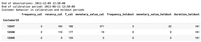

Training: BG/NBD Model

from lifetimes import BetaGeoFitter
#training: BG/NBD Model
bgf = lifetimes.BetaGeoFitter(penalizer_coef=1e-06)
bgf.fit(
        frequency = df_ch["frequency_cal"],
        recency = df_ch["recency_cal"],
        T = df_ch["T_cal"],
        weights = None,
        verbose = True)

Testing: predicted vs actual purchases in the holdout period

from lifetimes.plotting import plot_calibration_purchases_vs_holdout_purchases
#testing: predicted vs actual purchases in holdout period
fig = plt.figure(figsize=(7, 7))
plot_calibration_purchases_vs_holdout_purchases(bgf, df_ch)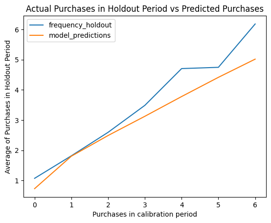

The plot above shows that our model does an excellent job of predicting the frequencies in the observation dataset.

Model Evaluation: BG/NBD Model

from sklearn.metrics import mean_squared_error

# Fill NaN values with 0
df_ch["n_transactions_holdout_real"].fillna(0, inplace=True)
df_ch["n_transactions_holdout_pred"].fillna(0, inplace=True)

# Compute RMSE
RMSE = mean_squared_error(y_true=df_ch["n_transactions_holdout_real"],
                          y_pred=df_ch["n_transactions_holdout_pred"],
                          squared=False)

RMSE 
#2.888243784621575

From the result, we get the root mean square error (RMSE), which is the standard deviation of the residuals (prediction errors): 2.888243784621575. The model's predictions deviate from the actual purchase frequencies by an average of approximately 2.8 units.

Based on our model evaluation results, which are good, we can conclude that our model is ready for prediction.

Predict the Future Number of Purchases using the BG/NBD Model

#Function to predict each customer's purchase over next t days
def predict_purch(df, t):
    df["predict_purch_" + str(t)] = \
        bgf.predict(
            t,
            df["frequency"],
            df["recency"],
            df["T"])

#Call function
t_FC = [90, 180, 270, 360]
_ = [predict_purch(df_rft, t) for t in t_FC]
pd.options.display.float_format = '{:,.1f}'.format
print("predicted number of purchases for each customer over next t days:")
pd.options.display.float_format = '{:,.0f}'.format
df_rft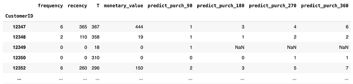

Our model tries to predict every customer's purchase over the next 90, 180, 270, and 360 days.

Probability of Being Alive

This method computes the probability that a customer with history (frequency, recency, T) is currently alive.

#Probability that a customer has not churned(='is alive')
#Based on customer's spesific recency r and frequency f
from lifetimes.plotting import plot_probability_alive_matrix
fig = plt.figure(figsize=(7,7))
plot_probability_alive_matrix(
                    model = bgf,
                    max_frequency = max_freq,
                    max_recency = max_rec,
                    cmap='inferno');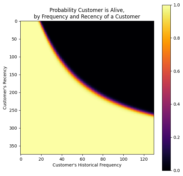

The probability of being alive is calculated based on the recency and frequency of a customer.

If a customer has bought multiple times (frequency) and the time between the first & last transaction is high (recency), their probability of being alive is high.

Similarly, if a customer has less frequency (bought once or twice) and the time between the first & last transaction is low (recency), their probability of being alive is high.

Predict the Monetary Value of Transactions using the Gamma-Gamma Model

#Select customers with monetary value > 0
df_rftv = df_rft[df_rft["monetary_value"]>0]
pd.options.display.float_format = '{:,.2f}'.format
df_rftv.describe()

We only use customer data from customers who made purchases with the business, meaning they are considered dead if they didn't purchase during the period.

Correlation Frequency and Monetary Value

corr_matrix = df_rftv[["monetary_value", "frequency"]].corr()
corr = corr_matrix.iloc[1,0]
print("Pearson correlation: %.3f" % corr)

# Pearson correlation: 0.036

The gamma-gamma Model requires a Pearson correlation close to 0 between purchase frequency and monetary value. The correlation on our dataset seems very weak, at 0.036. Therefore, we can conclude that the assumption is satisfied, and we can fit the model to our data.

Fitting Gamma-Gamma Model

from lifetimes import GammaGammaFitter

# Fine-tuning parameters
penalizer_coef = 1e-06
tolerance = 1e-06

# Fitting the Gamma-Gamma Model
ggf = GammaGammaFitter(penalizer_coef=penalizer_coef)
ggf.fit(
    frequency=df_rftv["frequency"],
    monetary_value=df_rftv["monetary_value"],
    weights=None,  # You may consider using weights if applicable
    verbose=True,
    tol=tolerance,  # Adjust tolerance level for convergence
    q_constraint=True
)

# Set display format
pd.options.display.float_format = '{:,.3f}'.format

# Display model summary
print(ggf.summary)

Estimate the average transaction value of each customer based on frequency and monetary value

from sklearn.metrics import mean_absolute_percentage_error
#Estimate the average transaction value of each customer, based on frequency and monetary value
exp_avg_rev = ggf.conditional_expected_average_profit(
                df_rftv["frequency"],
                df_rftv["monetary_value"])

df_rftv["exp_avg_rev"] = exp_avg_rev
df_rftv["avg_rev"] = df_rftv["monetary_value"]
df_rftv["error_rev"] = df_rftv["exp_avg_rev"] - df_rftv["avg_rev"]

mape = mean_absolute_percentage_error(exp_avg_rev, df_rftv["monetary_value"])
print("MAPE of predicted revenues: {:.2%}".format(mape))

pd.options.display.float_format = '{:,.3f}'.format
df_rftv.head()

# MAPE of predicted revenues: 15.74%

This method computes the conditional expectation of the average profit per transaction for a group of one or more customers. After checking the Mean Absolute Percentage Error (MAPE) between the expected average and actual monetary values, the MAPE of predicted revenues is 15.74%. The values seem okay.

Compute Customer Lifetime Value (CLV)

#Compute customer lifetime value
#DISCOUNT_a : annual discount rate
#LIFE : lifetime expected for the customers in months
DISCOUNT_a = 0.06
LIFE = 12

#Monthly discount rate
discount_m = (1 + DISCOUNT_a)**(1/12) - 1

#Expected customer lifetime values
clv = ggf.customer_lifetime_value(
        transaction_prediction_model = bgf,
        frequency = df_rftv["frequency"],
        recency = df_rftv["recency"],
        T = df_rftv["T"],
        monetary_value = df_rftv["monetary_value"],
        time = LIFE,
        freq = "D",
        discount_rate = discount_m)

# Check if 'CLV' already exists in the DataFrame
if 'CLV' in df_rftv.columns:
    # Drop the existing 'CLV' column
    df_rftv.drop(columns=['CLV'], inplace=True)

# Insert the new 'CLV' column
df_rftv.insert(0, "CLV", clv)

# Description of the DataFrame
df_rftv.describe().T

Finally, let's compute the CLV for each customer's next 12 months, assuming the discount rate per year is 6%.

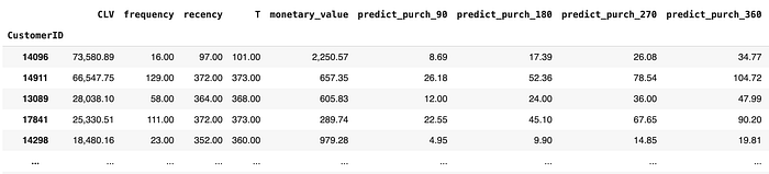
So, this is our prediction of customer lifetime value (CLV) using the Gamma-Gamma model. I integrated the CLV prediction with the result BG/NBD model, which predicts purchase, so that we can have more information about the prediction of our CLV.

From this result, we can do customer segmentation based on customer lifetime value using the K-Means algorithm.

CLV Segmentations

Find Optimal Clusters

from yellowbrick.cluster import KElbowVisualizer

#Instantiate the clustering model and visualizer
km_model = KMeans()
visualizer = KElbowVisualizer(km_model, k=(2,10))

visualizer.fit(df_rftv)
visualizer.show()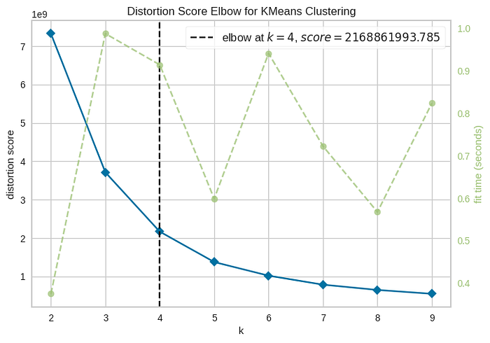

After calculating the optimal number of clusters using the elbow method, it has been decided that the most effective choice is k= 4. This will enable the segmentation of customers into four distinct categories.

Grouping by Clusters

#Grouping by clusters
df_clusters = df_rftv.groupby(['cluster'])['CLV']\
                    .agg(['mean', "count"])\
                    .reset_index()

df_clusters.columns = ["clusters", "avg_CLV", "n_customers"]

df_clusters['perct_customers'] = (df_clusters['n_customers']/df_clusters['n_customers']\
                                    .sum())*100

df_clusters

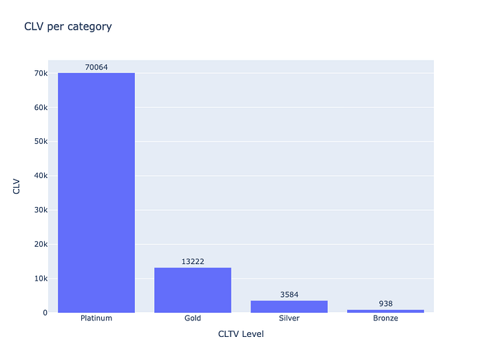
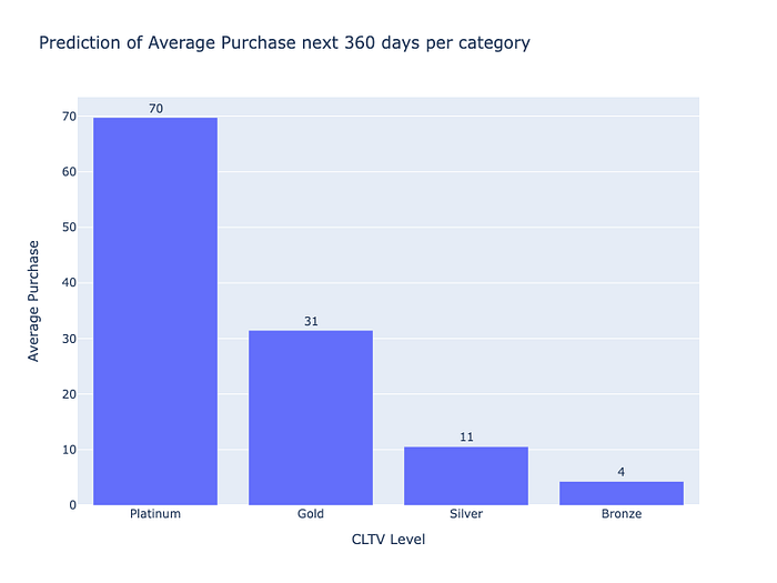
The table above shows that cluster 1 has the highest average CLV, representing (0.08%) with $70.064. We will name the cluster "Platinum," the second highest cluster 2, representing (0.72%) with an average CLV of $13.221. We will name the cluster "Gold," followed by cluster 3, representing (15.51%) with an average CLV of $3.583. We will name the cluster "Silver" and last, cluster 0 for the majority (83.70%) of customers with an average CLV of $937, we will name the cluster "Bronze."

#Rename the columns
df_rftv['CLTV_level'] = df_rftv['cluster']\
                            .replace({0:"Bronze", 1:"Platinum", 2:"Gold", 3:"Silver"})

Prediction of Average CLV next 12 months per Segmentation

Prediction of Average Purchase in the next 360 days per Segmentation

Combine RFM & CLV Results

Last, we can combine CLV results with RFM segmentation results to gain more information and make data-driven decisions about marketing strategy.

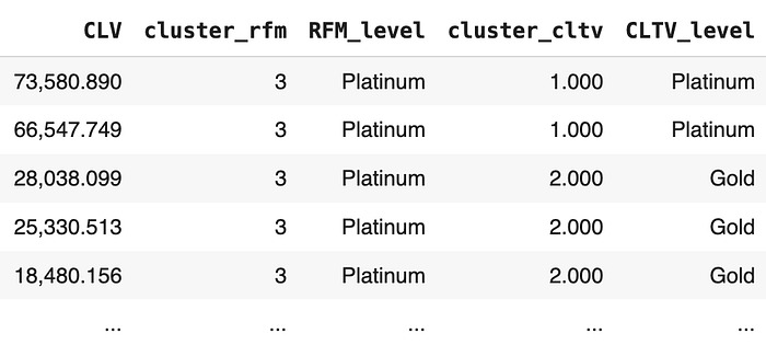
So, based on this table, we can use this data to see our customer segmentation based on historical data using RFM Segmentation, and we can see our prediction about customer segmentation using the CLV model.

Conclusion

The Customer Lifetime Value (CLV) model offers substantial benefits for businesses, including improved decision-making, enhanced customer retention, reduced acquisition costs, and increased profits over time. Predictive CLV, employing models like BG-NBD and Gamma-Gamma, forecasts future customer behavior and monetary value. The integration of these models enables businesses to segment customers effectively, allowing for tailored marketing strategies and data-driven decision-making to maximize profitability and customer satisfaction.

References:

Thank you for reading, and feel free to connect with me on LinkedIn

GitHub Link: https://github.com/Ishlafakhri/RFM-Customer-Segmentation